Polylogarithm
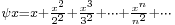
In mathematics, the polylogarithm (also known as Jonquière's function) is a special function Lis(z) that is defined by the infinite sum, or power series:
It is in general not an elementary function, unlike the related logarithm function. The above definition is valid for all complex values of the order s and the argument z where |z| < 1. The polylogarithm is defined over a larger range of z than the above definition allows by the process of analytic continuation.
 |
 |
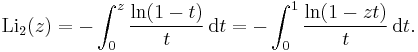
 |
 |
 |
 |
 |
The special case s = 1 involves the ordinary natural logarithm (Li1(z) = −ln(1−z)) while the special cases s = 2 and s = 3 are called the dilogarithm (also referred to as Spence's function) and trilogarithm respectively. The name of the function comes from the fact that it may alternatively be defined as the repeated integral of itself, namely that
Thus the dilogarithm is an integral of the logarithm, and so on. For nonpositive integer orders s, the polylogarithm is a rational function.
The polylogarithm also arises in the closed form of the integral of the Fermi–Dirac distribution and the Bose–Einstein distribution and is sometimes known as the Fermi–Dirac integral or the Bose–Einstein integral. Polylogarithms should not be confused with polylogarithmic functions nor with the offset logarithmic integral which has a similar notation.
Contents |
Properties
Preliminary note: In the important case where the polylogarithm order s is an integer, it will be represented by n (or −n when negative). It is often convenient to define μ = ln(z) where ln(z) is the principal branch of the complex logarithm Ln(z) so that −π < Im(μ) ≤ π. Also, all exponentiation will be assumed to be single-valued: zs = exp(s ln(z)).
Depending on the order s, the polylogarithm may be multi-valued. The principal branch of Lis(z) is taken to be that given for |z| < 1 by the above series definition and taken to be continuous except on the positive real axis, where a cut is made from z = 1 to ∞ such that axis is placed on the lower half plane of z. In terms of μ, this amounts to −π < arg(−μ) ≤ π. The discontinuity of the polylogarithm in dependence on μ can sometimes be confusing.
For real argument z, the polylogarithm of real order s is real if z < 1, and its imaginary part for z ≥ 1 is (Wood 1992, § 3):
Going across the cut, if δ is an infinitesimally small positive real number, then:

Both can be concluded from the series expansion (see below) of Lis(eµ) about µ = 0.
The derivatives of the polylogarithm follow from the defining power series:


The square relationship is easily seen from the duplication formula (see also (Clunie 1954), (Schrödinger 1952)):

Note that Kummer's function obeys a very similar duplication formula. This is a special case of the multiplication formula, for any integer p:

which can be proved using the series definition of the polylogarithm and the orthogonality of the exponential terms (e.g. see discrete Fourier transform).
Another important property, the inversion formula, involves the Hurwitz zeta function or the Bernoulli polynomials and is found under relationship to other functions below.
Particular values
For particular cases, the polylogarithm may be expressed in terms of other functions (see below). Particular values for the polylogarithm may thus be found as particular values of these other functions.
1. For integer values of the polylogarithm order, the following explicit expressions are obtained by repeated application of z·∂/∂z to Li1(z):


Accordingly the polylogarithm reduces to a ratio of polynomials in z, and is therefore a rational function of z, for all nonpositive integer orders. The general case may be expressed as a finite sum:

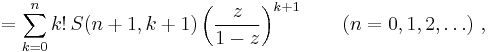
where S(n,k) are the Stirling numbers of the second kind. Equivalent formulae applicable to negative integer orders are (Wood 1992, § 6):

and:

where  are the Eulerian numbers. All roots of Li−n(z) are distinct and real; they include z = 0, while the remainder is negative and centered about z = −1 on a logarithmic scale. As n becomes large, the numerical evaluation of these rational expressions increasingly suffers from cancellation (Wood 1992, § 6); full accuracy can be obtained, however, by computing Li−n(z) via the general relation with the Hurwitz zeta function (see below).
2. Some particular expressions for half-integer values of the argument z are:
![\operatorname{Li}_2(\tfrac12) = \tfrac1{12}[\pi^2-6(\ln 2)^2]](/2012-wikipedia_en_all_nopic_01_2012/I/3f0cc7fb975d81ecf9d816801cded63f.png)
![\operatorname{Li}_3(\tfrac12) = \tfrac1{24}[4(\ln 2)^3-2\pi^2 \ln 2%2B21\,\zeta(3)]](/2012-wikipedia_en_all_nopic_01_2012/I/b9115f70020130a11716ad3c7a0251ba.png)
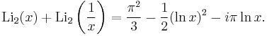
where ζ is the Riemann zeta function. No formulae of this type are known for higher integer orders (Lewin 1991, p. 2). However, one has for instance:

involving the alternating double sum  (CITATION REQUIRED!).
3. As a straightforward consequence of the series definition, values of the polylogarithm at the pth complex roots of unity are given by the Fourier sum:
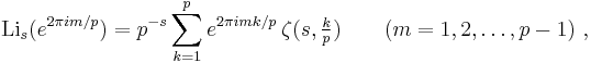
where ζ is the Hurwitz zeta function. For Re(s) > 1, where Lis(1) is finite, the relation also holds with m = 0 or m = p. While this formula is not as simple as that implied by the more general relation with the Hurwitz zeta function listed under relationship to other functions below, it has the advantage of applying to positive integer values of s as well. As usual, the relation may be inverted to express ζ(s, m⁄p) for any m = 1, ..., p as a Fourier sum of Lis(exp(2πi k⁄p)) over k = 1, ..., p.
Relationship to other functions
- For z = 1 the polylogarithm reduces to the Riemann zeta function

- The polylogarithm is related to Dirichlet eta function and the Dirichlet beta function:

- where η(s) is the Dirichlet eta function. For pure imaginary arguments, we have:

- where β(s) is the Dirichlet beta function.
- The polylogarithm is related to the complete Fermi–Dirac integral as:

- The polylogarithm is a special case of the incomplete polylogarithm function

- The polylogarithm is a special case of the Lerch Transcendent (Erdélyi 1981, § 1.11-14)
- The polylogarithm is related to the Hurwitz zeta function by:
![\operatorname{Li}_s(z) = {\Gamma(1 \!-\! s) \over (2\pi)^{1-s}} \left[i^{1-s} ~\zeta \!\left(1 \!-\! s, ~\frac{1}{2} %2B {\ln(-z) \over {2\pi i}} \right) %2B i^{s-1} ~\zeta \!\left(1 \!-\! s, ~\frac{1}{2} - {\ln(-z) \over {2\pi i}} \right) \right] ,](/2012-wikipedia_en_all_nopic_01_2012/I/58f08221c31b7d5c215a176f9c3b92e4.png)
- where Γ(1−s) is the gamma function, which causes the relation to fail for positive integer s; a derivation of this formula is given under series representations below. The polylogarithm is consequently also related to the Hurwitz zeta function by (Jonquière 1889):

- which holds for 0 ≤ Re(x) < 1 if Im(x) ≥ 0, and for 0 < Re(x) ≤ 1 if Im(x) < 0. Equivalently, for all complex s and for complex z ∉ ]0;1], the inversion formula reads

- and for all complex s and for complex z ∉ ]1;∞[

- These relations furnish the analytic continuation of the polylogarithm beyond the circle of convergence |z| = 1 of the defining power series. (Note that Erdélyi's corresponding equation (Erdélyi 1981, § 1.11-16) is not correct if one assumes that the principal branches of the polylogarithm and the logarithm are used simultaneously.) See below for a simplified formula when s is an integer.
- For positive integer polylogarithm orders s, the Hurwitz zeta function ζ(1−s, x) reduces to Bernoulli polynomials, ζ(1−n, x) = −Bn(x) / n, and Jonquière's inversion formula for n = 1, 2, 3, ... becomes:

- where again 0 ≤ Re(x) < 1 if Im(x) ≥ 0, and 0 < Re(x) ≤ 1 if Im(x) < 0. Upon restriction of the polylogarithm argument to the unit circle, Im(x) = 0, the left hand side of this formula simplifies to 2 Re(Lin(e2πix)) if n is even, and to 2i Im(Lin(e2πix)) if n is odd. For negative integer orders, on the other hand, the divergence of Γ(s) implies for all z that (Erdélyi 1981, § 1.11-17):

- More generally one has for n = 0, ±1, ±2, ±3, ... :
![\operatorname{Li}_{n}(z) %2B (-1)^n \,\operatorname{Li}_{n}(1/z) = -\frac{(2\pi i)^n}{n!} ~B_n \!\left( \frac{1}{2} %2B {\ln(-z) \over {2\pi i}} \right) \qquad (z ~\not\in ~]0;1]) \,,](/2012-wikipedia_en_all_nopic_01_2012/I/eec06963c5905b4097756c96744ceb13.png)
![\operatorname{Li}_{n}(z) %2B (-1)^n \,\operatorname{Li}_{n}(1/z) = -\frac{(2\pi i)^n}{n!} ~B_n \!\left( \frac{1}{2} - {\ln(-1/z) \over {2\pi i}} \right) \qquad (z ~\not\in ~]1;\infty[) \,.](/2012-wikipedia_en_all_nopic_01_2012/I/95e18ee66c99f62f25f6fe76b72de40a.png)
- (Note that the corresponding equation (Erdélyi 1981, § 1.11-18) is again not correct.)
- The polylogarithm with pure imaginary μ may be expressed in terms of the Clausen functions Cis(θ) and Sis(θ), and vice versa (Lewin 1958, Ch. VII § 1.4), (Abramowitz & Stegun 1972, § 27.8):

- The inverse tangent integral Tis(z) (Lewin 1958, Ch. VII § 1.2) can be expressed in terms of polylogarithms:
![Ti_s(z) = {1 \over 2i} \left[ \operatorname{Li}_s(i z) - \operatorname{Li}_s(-i z) \right] .](/2012-wikipedia_en_all_nopic_01_2012/I/e5bc55ead821213f5724503d7f8f875b.png)
- The relation in particular implies:


- which explains the function name.
- The Legendre chi function χs(z) (Lewin 1958, Ch. VII § 1.1), (Boersma 1992) can be expressed in terms of polylogarithms:
![\chi_s(z) = \tfrac {1}{2} \left[ \operatorname{Li}_s(z) - \operatorname{Li}_s(-z) \right] .](/2012-wikipedia_en_all_nopic_01_2012/I/b4fd253d5440f20209a7438de6005848.png)
- The polylogarithm of integer order can be expressed as a generalized hypergeometric function:


- In terms of the incomplete zeta functions or "Debye functions" (Abramowitz & Stegun 1972, § 27.1):
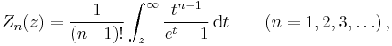
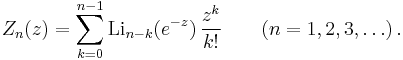
- the polylogarithm Lin(z) for positive integer n may be expressed as the finite sum (Wood 1992, § 16):

- A remarkably similar expression relates the function Zn(z) to the polylogarithm:
Integral representations
Any of the following integral representations furnishes the analytic continuation of the polylogarithm beyond the circle of convergence |z| = 1 of the defining power series.
- The integral of the Bose–Einstein distribution is expressed in terms of a polylogarithm:
- This converges for Re(s) > 0 and all z except for z real and ≥ 1. The polylogarithm in this context is sometimes referred to as a Bose integral or a Bose-Einstein integral.
- The integral of the Fermi-Dirac distribution is also expressed in terms of a polylogarithm:

- This converges for Re(s) > 0 and all z except for z real and ≤ −1. The polylogarithm in this context is sometimes referred to as a Fermi integral or a Fermi–Dirac integral (GSL 2010).
- A complementary integral representation applies to Re(s) < 0 and to all z except to z real and ≥ 0:
![\operatorname{Li}_{s}(z) =
\int_0^\infty {t^{-s} \,\sin[s \,\pi /2 - t \ln(-z)] \over \sinh(\pi t)} \,\mathrm{d}t.](/2012-wikipedia_en_all_nopic_01_2012/I/76bbde89650bac5606758ecc012c8d80.png)
- This integral follows from the general relation of the polylogarithm with the Hurwitz zeta function (see above) and a familiar integral representation of the latter.
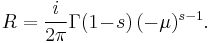
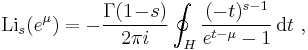
- The polylogarithm may be rather generally represented by a Hankel contour integral (Whittaker & Watson 1952, § 12.22, § 13.13). As long as the t = μ pole of the integrand does not lie on the non-negative real axis, and s ≠ 1, 2, 3, ..., we have:

- where H represents the Hankel contour. The integrand has a cut along the real axis from zero to infinity, with the axis belonging to the lower half plane of t. The integration starts at +∞ on the upper half plane (Im(t) > 0), circles the origin without enclosing any of the poles t = µ + 2kπi, and terminates at +∞ on the lower half plane (Im(t) < 0). For the case where µ is real and non-negative, we can simply subtract the contribution of the enclosed t = µ pole:

- where R is the residue of the pole:
- A Hermite-like integral representation valid for all complex z and for all complex s is:

- where Γ is the upper incomplete gamma-function. Note that all (but not part) of the ln(z) in this expression can be replaced by −ln(1⁄z). A related representation which also holds for all complex s,
![\operatorname{Li}_s(z) = {z\over2} %2B z \int_0^\infty \frac{\sin[s \arctan t \,- \,t \ln(-z)]} {(1%2Bt^2)^{s/2} \,\sinh(\pi t)} \,\mathrm{d}t,](/2012-wikipedia_en_all_nopic_01_2012/I/770b45e094318c51aa16d2a634e2ef25.png)
- avoids the use of the incomplete gamma function, but this integral fails for z on the positive real axis.
Series representations
1. As noted under integral representations above, the Bose-Einstein integral representation of the polylogarithm may be extended to negative orders s by means of Hankel contour integration:
where H is the Hankel contour, s ≠ 1, 2, 3, ..., and the t = μ pole of the integrand does not lie on the non-negative real axis. The contour can be modified so that it encloses the poles of the integrand at t − µ = 2kπi, and the integral can be evaluated as the sum of the residues (Wood 1992, § 12, 13), (Gradshteyn & Ryzhik 1980, § 9.553):

This will hold for Re(s) < 0 and all μ except where eμ = 1. For 0 < Im(µ) ≤ 2π the sum can be split as:
![\operatorname{Li}_s(e^\mu) = \Gamma(1-s) \left[ (-2\pi i)^{s-1} \sum_{k=0}^\infty \left(k %2B {\mu \over {2\pi i}} \right)^{s-1} %2B (2\pi i)^{s-1} \sum_{k=0}^\infty \left(k%2B1- {\mu \over {2\pi i}} \right)^{s-1} \right] ,](/2012-wikipedia_en_all_nopic_01_2012/I/342b40f32d337c2862bc4a0b04ed4144.png)
where the two series can now be identified with the Hurwitz zeta function:
![\operatorname{Li}_s(e^\mu) = {\Gamma(1 \!-\! s) \over (2\pi)^{1-s}} \left[i^{1-s} ~\zeta \!\left(1 \!-\! s, ~{\mu \over {2\pi i}} \right) %2B i^{s-1} ~\zeta \!\left(1 \!-\! s, ~1 - {\mu \over {2\pi i}} \right) \right]
\qquad (0 < \textrm{Im}(\mu) \leq 2\pi) ~.](/2012-wikipedia_en_all_nopic_01_2012/I/0998c6ebc872f786a2e277773a82bae2.png)
This relation, which has already been given under relationship to other functions above, holds for all complex s ≠ 1, 2, 3, ... and was first derived in (Jonquière 1889).
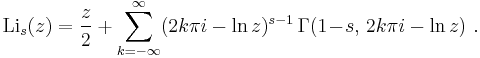
2. In order to represent the polylogarithm as a power series about µ = 0, we write the series derived from the Hankel contour integral as:
![\operatorname{Li}_s(e^\mu) = \Gamma(1 \!-\! s) \,(-\mu)^{s-1} %2B \sum_{h=1}^\infty \left[(-2 h \pi i - \mu)^{s-1} %2B (2 h \pi i - \mu)^{s-1} \right] .](/2012-wikipedia_en_all_nopic_01_2012/I/2c36571ee0e532e01a9613a3f3aa14d3.png)
When the binomial powers in the sum are expanded about µ = 0 and the order of summation is reversed, the sum over h can be expressed in closed form:

This result holds for |µ| < 2π and, thanks to the analytic continuation provided by the zeta functions, for all s ≠ 1, 2, 3, ... . If the order s is a positive integer, n, both the term with k = n − 1 and the gamma function become infinite, although their sum does not. One obtains (Wood 1992, § 9), (Gradshteyn & Ryzhik 1980, § 9.554):
![\lim_{s \rightarrow k%2B1} \left[ {\zeta(s-k) \over k!} \,\mu^k %2B \Gamma(1 \!-\! s) \,(-\mu)^{s-1} \right] = {\mu^k \over k!} \left[ \,\sum_{h=1}^k {1 \over h} - \ln(-\mu) \right] ,](/2012-wikipedia_en_all_nopic_01_2012/I/742765859a01ce0e3e4a72521769a3b7.png)
where the sum over h vanishes if k = 0. So, for s = n where n is a positive integer and for |μ| < 2π we have the series:
![\operatorname{Li}_{n}(e^\mu) = {\mu^{n-1} \over (n \!-\! 1)!} \left[ H_{n-1} - \ln(-\mu) \right] %2B \sum_{k=0,\,k\ne n-1}^\infty {\zeta(n-k) \over k!} \,\mu^k ~,](/2012-wikipedia_en_all_nopic_01_2012/I/094dd9b2373738ca3f072c936015e2a6.png)
where Hn denotes the nth harmonic number:

The problem terms now contain −ln(−μ) which, when multiplied by μn−1, will tend to zero as μ → 0, except for n = 1. This reflects the fact that there is a true logarithmic singularity in Lis(z) at s = 1 and z = 1 since:

For s close, but not equal, to a positive integer, the divergent terms in the expansion about µ = 0 can be expected to cause computational difficulties (Wood 1992, § 9). Note also that Erdélyi's corresponding expansion (Erdélyi 1981, § 1.11-15) in powers of ln(z) is not correct if one assumes that the principal branches of the polylogarithm and the logarithm are used simultaneously, since ln(1⁄z) is not uniformly equal to −ln(z).
For nonpositive integer values of s, the zeta function ζ(s − k) in the expansion about µ = 0 reduces to Bernoulli numbers: ζ(−n − k) = −B1+n+k / (1 + n + k). Numerical evaluation of Li−n(z) by this series does not suffer from the cancellation effects that the finite rational expressions given under particular values above exhibit for large n.
3. By use of the identity

the Bose-Einstein integral representation of the polylogarithm (see above) may be cast in the form:

Replacing the hyperbolic cotangent with a bilateral series,

then reversing the order of integral and sum, and finally identifying the summands with an integral representation of the upper incomplete gamma function, one obtains:
For both the bilateral series of this result and that for the hyperbolic cotangent, symmetric partial sums from −kmax to kmax converge unconditionally as kmax → ∞. Provided the summation is performed symmetrically, this series for Lis(z) thus holds for all complex s as well as all complex z.
4. Introducing an explicit expression for the Stirling numbers of the second kind into the finite sum for the polylogarithm of nonpositive integer order (see above) one may write:

The infinite series obtained by simply extending the outer summation to ∞ (Guillera & Sondow 2008, Theorem 2.1):
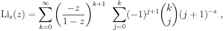
turns out to converge to the polylogarithm for all complex s and for complex z with Re(z) < 1⁄2, as can be verified for |−z⁄(1−z)| < 1⁄2 by reversing the order of summation and using:
![\sum_{k=j}^\infty {k \choose j} \left( {-z \over 1-z} \right)^{k%2B1} = \left[ \left( {-z \over 1-z} \right)^{-1} -1 \right]^{-j-1} = (-z)^{j%2B1} ~.](/2012-wikipedia_en_all_nopic_01_2012/I/022c5bae44cd100f406be7556be6d90c.png)
For the other arguments with Re(z) < 1⁄2 the result follows by analytic continuation. This procedure is equivalent to applying Euler's transformation to the series in z that defines the polylogarithm.
Asymptotic expansions
For |z| ≫ 1, the polylogarithm can be expanded into asymptotic series in terms of ln(−z):
![\operatorname{Li}_s(z) = {\pm i\pi \over \Gamma(s)} \,[\ln(-z) \pm i\pi]^{s-1} - \sum_{k = 0}^\infty (-1)^k \,(2\pi)^{2k} \,{B_{2k} \over (2 k)!} \,{[\ln(-z) \pm i\pi]^{s-2 k} \over \Gamma(s%2B1-2k)} ~,](/2012-wikipedia_en_all_nopic_01_2012/I/251b3f5e35387dad674da52eb29d3d99.png)
![\operatorname{Li}_s(z) = \sum_{k = 0}^\infty (-1)^k \,(1-2^{1-2k}) \,(2\pi)^{2k} \,{B_{2k} \over (2k)!} \,{[\ln(-z)]^{s-2 k} \over \Gamma(s%2B1-2k)} ~,](/2012-wikipedia_en_all_nopic_01_2012/I/b0f69a3ec7d1b9de967f3bad1b39f4f9.png)
where B2k are the Bernoulli numbers. Both versions hold for all s and for any arg(z). As usual, the summation should be terminated when the terms start growing in magnitude. For negative integer s, the expansions vanish entirely; for non-negative integer s, they break off after a finite number of terms. Wood (1992, § 11) describes a method for obtaining these series from the Bose-Einstein integral representation (note that his equation 11.2 for Lis(eµ) requires −2π < Im(µ) ≤ 0).
Limiting behavior
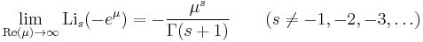
The following limits result from the various representations of the polylogarithm (Wood 1992, § 22):


Dilogarithm
The dilogarithm is just the polylogarithm with s = 2. An alternate integral expression for the dilogarithm for arbitrary complex z is (Abramowitz & Stegun 1972, § 27.7):
A source of confusion is that some computer algebra systems define the dilogarithm as dilog(z) = Li2(1−z).
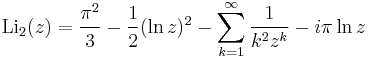
In the case of real z ≥ 1 the first integral expression for the dilogarithm can be written as
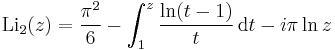
from which expanding ln(t−1) and integrating term by term we obtain
The Abel identity for the dilogarithm is given by (Abel 1881)

for x ∉ ]1;∞[ and y ∉ ]1;∞[.
This is immediately seen to hold for either x = 0 or y = 0, and for general arguments is then easily verified by differentiation ∂/∂x ∂/∂y. For y = 1−x the identity reduces to Euler's reflection formula

where Li2(1) = ζ(2) = 1⁄6 π2 has been used.
In terms of the new variables u = x/(1−y), v = y/(1−x) the Abel identity reads

which corresponds to the pentagon identity given in (Rogers 1907).
From the Abel identity for y = x and the square relationship we have Landen's identity
![\operatorname{Li}_2(-x) = -\operatorname{Li}_2 \left( \frac{x}{1%2Bx} \right) - \frac{1}{2} [\ln(x%2B1)]^2 \qquad (x \not \in ~]-\infty;-1[),](/2012-wikipedia_en_all_nopic_01_2012/I/270969b261d2b3a769591ae06bdf01a6.png)
and the inversion formula for the dilogarithm reads
![\operatorname{Li}_2(x) %2B \operatorname{Li}_2 \left( \frac{1}{x} \right) = -\frac{\pi^2}{6} - \frac{1}{2} [\ln(-x)]^2 \qquad (x \not \in ~]0;1[),](/2012-wikipedia_en_all_nopic_01_2012/I/0e52d83d31868607f02d11e970590a58.png)
and for x ≥ 1 also
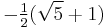
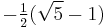
Known closed-form evaluations of the dilogarithm at special arguments are collected in the table below. Arguments in the first column are related by reflection x ↔ 1−x or inversion x ↔ 1⁄x to either x = 0 or x = −1; arguments in the third column are all interrelated by these operations.
Historical note: Don Zagier (1989) remarked that "The dilogarithm is the only mathematical function with a sense of humor".
-
Special values of the dilogarithm 


![-\tfrac {1}{10} \pi^2 - \ln^2[\tfrac {1}{2} (\sqrt 5 - 1)] \,](/2012-wikipedia_en_all_nopic_01_2012/I/82051cb652fef5498028a0e27be7cb65.png)

![-\tfrac {1}{15} \pi^2 %2B \tfrac {1}{2} \ln^2[\tfrac {1}{2} (\sqrt 5 - 1)] \,](/2012-wikipedia_en_all_nopic_01_2012/I/e2c36cac3f5b099853864d6c4fe8a841.png)

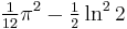

![\tfrac {1}{15} \pi^2 - \ln^2[\tfrac {1}{2} (\sqrt 5 - 1)] \,](/2012-wikipedia_en_all_nopic_01_2012/I/cf9e07a7efd5b8c5e0bf83ae10b936cd.png)


![\tfrac {1}{10} \pi^2 - \ln^2[\tfrac {1}{2} (\sqrt 5 - 1)] \,](/2012-wikipedia_en_all_nopic_01_2012/I/7e0d6d0e021635f42cdbed39120fce84.png)


![\tfrac {11}{15} \pi^2 %2B \tfrac {1}{2} \ln^2[-\tfrac{1}{2} (\sqrt 5 - 1)] \,](/2012-wikipedia_en_all_nopic_01_2012/I/4b11c9801fd645e7aea2322e2c5edf50.png)

![-\tfrac {11}{15} \pi^2 - \ln^2[-\tfrac {1}{2} (\sqrt 5 - 1)] \,](/2012-wikipedia_en_all_nopic_01_2012/I/9fc5f4c8078ddde9e2cf5f252d7ada78.png)
Polylogarithm ladders
Leonard Lewin discovered a remarkable and broad generalization of a number of classical relationships on the polylogarithm for special values. These are now called polylogarithm ladders. Define  as the reciprocal of the golden ratio. Then two simple examples of results from ladders are


given by Landen. Polylogarithm ladders occur naturally and deeply in K-theory and algebraic geometry. Polylogarithm ladders provide the basis for the rapid computations of various mathematical constants by means of the BBP algorithm (Bailey, Borwein & Plouffe 1997).
Monodromy
The polylogarithm has two branch points; one at z = 1 and another at z = 0. The second branch point, at z = 0, is not visible on the main sheet of the polylogarithm; it becomes visible only when the function is analytically continued to its other sheets. The monodromy group for the polylogarithm consists of the homotopy classes of loops that wind around the two branch points. Denoting these two by m0 and m1, the monodromy group has the group presentation

For the special case of the dilogarithm, one also has that wm0 = m0w, and the monodromy group becomes the Heisenberg group (identifying m0, m1 and w with x, y, z) (Vepstas 2007).
References
- Abel, N.H. (1881) [1826]. "Note sur la fonction
 ". In Sylow, L.; Lie, S. (in French) (PDF). Œuvres complètes de Niels Henrik Abel − Nouvelle édition, Tome II. Christiania [Oslo]: Grøndahl & Søn. pp. 189–193. http://www.abelprisen.no/verker/oeuvres_1881_del2/oeuvres_completes_de_abel_nouv_ed_2_kap14_opt.pdf. (this 1826 manuscript was only published posthumously.)
 - Abramowitz, M.; Stegun, I.A. (1972). Handbook of Mathematical Functions with Formulas, Graphs, and Mathematical Tables. New York: Dover Publications. ISBN 0-486-61272-4.
- Apostol, T.M. (2010), "Polylogarithm", in Olver, Frank W. J.; Lozier, Daniel M.; Boisvert, Ronald F. et al., NIST Handbook of Mathematical Functions, Cambridge University Press, ISBN 978-0521192255, MR2723248, http://dlmf.nist.gov/25.12
- Bailey, D.H.; Borwein, P.B.; Plouffe, S. (April 1997). "On the Rapid Computation of Various Polylogarithmic Constants" (PDF). Mathematics of Computation 66 (218): 903–913. doi:10.1090/S0025-5718-97-00856-9. http://crd.lbl.gov/~dhbailey/dhbpapers/digits.pdf.
- Bailey, D.H.; Broadhurst, D.J. (June 20, 1999). "A Seventeenth-Order Polylogarithm Ladder". arXiv:math.CA/9906134 [math.CA].
- Berndt, B.C. (1994). Ramanujan's Notebooks, Part IV. New York: Springer-Verlag. pp. 323–326. ISBN 0-387-94109-6.
- Boersma, J.; Dempsey, J.P. (1992). "On the evaluation of Legendre's chi-function". Mathematics of Computation 59 (199): 157–163. doi:10.2307/2152987. JSTOR 2152987.
- Borwein, J.M.; Bradley, D.M.; Broadhurst, D.J.; Lisonek, P. (2001). "Special Values of Multiple Polylogarithms". Transactions of the American Mathematical Society 353 (3): 907–941. doi:10.1090/S0002-9947-00-02616-7.
- Clunie, J. (1954). "On Bose-Einstein functions". Proceedings of the Physical Society, Section A 67 (7): 632–636. doi:10.1088/0370-1298/67/7/308.
- Cohen, H.; Lewin, L.; Zagier, D. (1992). "A Sixteenth-Order Polylogarithm Ladder" (PS). Experimental Mathematics 1 (1): 25–34. http://www.expmath.org/expmath/volumes/1/1.html.
- Coxeter, H.S.M. (1935). "The functions of Schläfli and Lobatschefsky". Quarterly Journal of Mathematics (Oxford) 6 (1): 13–29. doi:10.1093/qmath/os-6.1.13.
- Cvijovic, D.; Klinowski, J. (1997). "Continued-fraction expansions for the Riemann zeta function and polylogarithms" (PDF). Proceedings of the American Mathematical Society 125 (9): 2543–2550. doi:10.1090/S0002-9939-97-04102-6. http://www.ams.org/journals/proc/1997-125-09/S0002-9939-97-04102-6/S0002-9939-97-04102-6.pdf.
- Cvijovic, D. (2007). "New integral representations of the polylogarithm function" (PDF). Proceedings of the Royal Society (London), Series A 463 (2080): 897–905. doi:10.1098/rspa.2006.1794. http://rspa.royalsocietypublishing.org/content/463/2080/897.full.pdf.
- Erdélyi, A.; Magnus, W.; Oberhettinger, F.; Tricomi, F.G. (1981). Higher Transcendental Functions, Vol. 1. New York: Krieger.
- Fornberg, B.; Kölbig, K.S. (1975). "Complex zeros of the Jonquiére or polylogarithm function". Mathematics of Computation 29 (130): 582–599. doi:10.2307/2005579. JSTOR 2005579.
- GNU Scientific Library (2010). "Reference Manual". http://www.gnu.org/software/gsl/manual/gsl-ref.html#SEC117. Retrieved 2010-06-13.
- Gradshteyn, I.S.; Ryzhik, I.M. (1980). Tables of Integrals, Series, and Products (4th ed.). New York: Academic Press. ISBN 0-12-294760-6.
- Guillera, J.; Sondow, J. (2008). "Double integrals and infinite products for some classical constants via analytic continuations of Lerch's transcendent". The Ramanujan Journal 16 (3): 247–270. arXiv:math.NT/0506319. doi:10.1007/s11139-007-9102-0.
- Hain, R.M. (March 25, 1992). "Classical polylogarithms". arXiv:alg-geom/9202022 [alg-geom].
- Jahnke, E.; Emde, F. (1945). Tables of Functions with Formulae and Curves (4th ed.). New York: Dover Publications.
- Jonquière, A. (1889). "Note sur la série
 " (in French) (PDF). Bulletin de la Société Mathématique de France 17: 142–152. http://archive.numdam.org/item?id=BSMF_1889__17__142_1.
 - Kölbig, K.S.; Mignaco, J.A.; Remiddi, E. (1970). "On Nielsen's generalized polylogarithms and their numerical calculation". BIT 10: 38–74. doi:10.1007/BF01940890.
- Kirillov, A.N. (1995). "Dilogarithm identities". Progress of Theoretical Physics Supplement 118: 61–142. arXiv:hep-th/9408113. doi:10.1143/PTPS.118.61.
- Lewin, L. (1958). Dilogarithms and Associated Functions. London: Macdonald. MR0105524.
- Lewin, L. (1981). Polylogarithms and Associated Functions. New York: North-Holland. ISBN 0-444-00550-1.
- Lewin, L. (Ed.) (1991). Structural Properties of Polylogarithms. Mathematical Surveys and Monographs. 37. Providence, RI: Amer. Math. Soc.. ISBN 0-8218-1634-9.
- Markman, B. (1965). "The Riemann Zeta Function". BIT 5: 138–141.
- Maximon, L.C. (2003). "The Dilogarithm Function for Complex Argument" (PDF). Proceedings of the Royal Society (London), Series A 459 (2039): 2807–2819. doi:10.1098/rspa.2003.1156. http://rspa.royalsocietypublishing.org/content/459/2039/2807.full.pdf.
- McDougall, J.; Stoner, E.C. (1938). "The computation of Fermi-Dirac functions". Philosophical Transactions of the Royal Society (London), Series A 237 (773): 67–104. doi:10.1098/rsta.1938.0004.
- Nielsen, N. (1909). "Der Eulersche Dilogarithmus und seine Verallgemeinerungen" (in German). Nova Acta Leopoldina (Halle – Leipzig, Germany: Kaiserlich-Leopoldinisch-Carolinische Deutsche Akademie der Naturforscher) XC (3): 121–212.
- Prudnikov, A.P.; Marichev, O.I.; Brychkov, Yu.A. (1990). Integrals and Series, Vol. 3: More Special Functions. Newark, NJ: Gordon and Breach. ISBN 2881246826. (see § 1.2, "The generalized zeta function, Bernoulli polynomials, Euler polynomials, and polylogarithms", p. 23.)
- Robinson, J.E. (1951). "Note on the Bose-Einstein integral functions". Physical Review, Series 2 83 (3): 678–679. doi:10.1103/PhysRev.83.678.
- Rogers, L.J. (1907). "On function sum theorems connected with the series
 ". Proceedings of the London Mathematical Society (2) 4 (1): 169–189. doi:10.1112/plms/s2-4.1.169.
 - Schrödinger, E. (1952). Statistical Thermodynamics (2nd ed.). Cambridge, UK: Cambridge University Press.
- Truesdell, C. (1945). "On a function which occurs in the theory of the structure of polymers". Annals of Mathematics, Series 2 46 (1): 144–157. doi:10.2307/1969153. JSTOR 1969153.
- Vepstas, L. (February 2007). "An efficient algorithm for accelerating the convergence of oscillatory series, useful for computing the polylogarithm and Hurwitz zeta functions". Numerical Algorithms 47 (3): 211. arXiv:math.CA/0702243. doi:10.1007/s11075-007-9153-8. (see also Numerical Algorithms 47 (2008), pp. 211–252.)
- Whittaker, E.T.; Watson, G.N. (1952). A Course of Modern Analysis (4th ed.). Cambridge, UK: Cambridge University Press.
- Wood, D.C. (June 1992). "The Computation of Polylogarithms. Technical Report 15-92*" (PS). Canterbury, UK: University of Kent Computing Laboratory. http://www.cs.kent.ac.uk/pubs/1992/110. Retrieved 2005-11-01.
- Zagier, D. (1989). "The dilogarithm function in geometry and number theory". Number Theory and Related Topics: papers presented at the Ramanujan Colloquium, Bombay, 1988. Studies in Mathematics. 12. Bombay: Tata Institute of Fundamental Research and Oxford University Press. pp. 231–249. ISBN 0-19-562367-3. (also appeared as "The remarkable dilogarithm" in Journal of Mathematical and Physical Sciences 22 (1988), pp. 131–145, and as Chapter I of (Zagier 2007).)
- Zagier, D. (2007). "The Dilogarithm Function". In Cartier, P.; Julia, B.; Moussa, P. et al. (PDF). Frontiers in Number Theory, Physics, and Geometry II – On Conformal Field Theories, Discrete Groups and Renormalization. Berlin: Springer-Verlag. pp. 3–65. ISBN 978-3-540-30307-7. http://mathlab.snu.ac.kr/~top/articles/zagier.pdf.
External links
- Weisstein, Eric W., "Polylogarithm" from MathWorld.
- Weisstein, Eric W., "Dilogarithm" from MathWorld.